
Generating large magnetic fields with superconducting coils
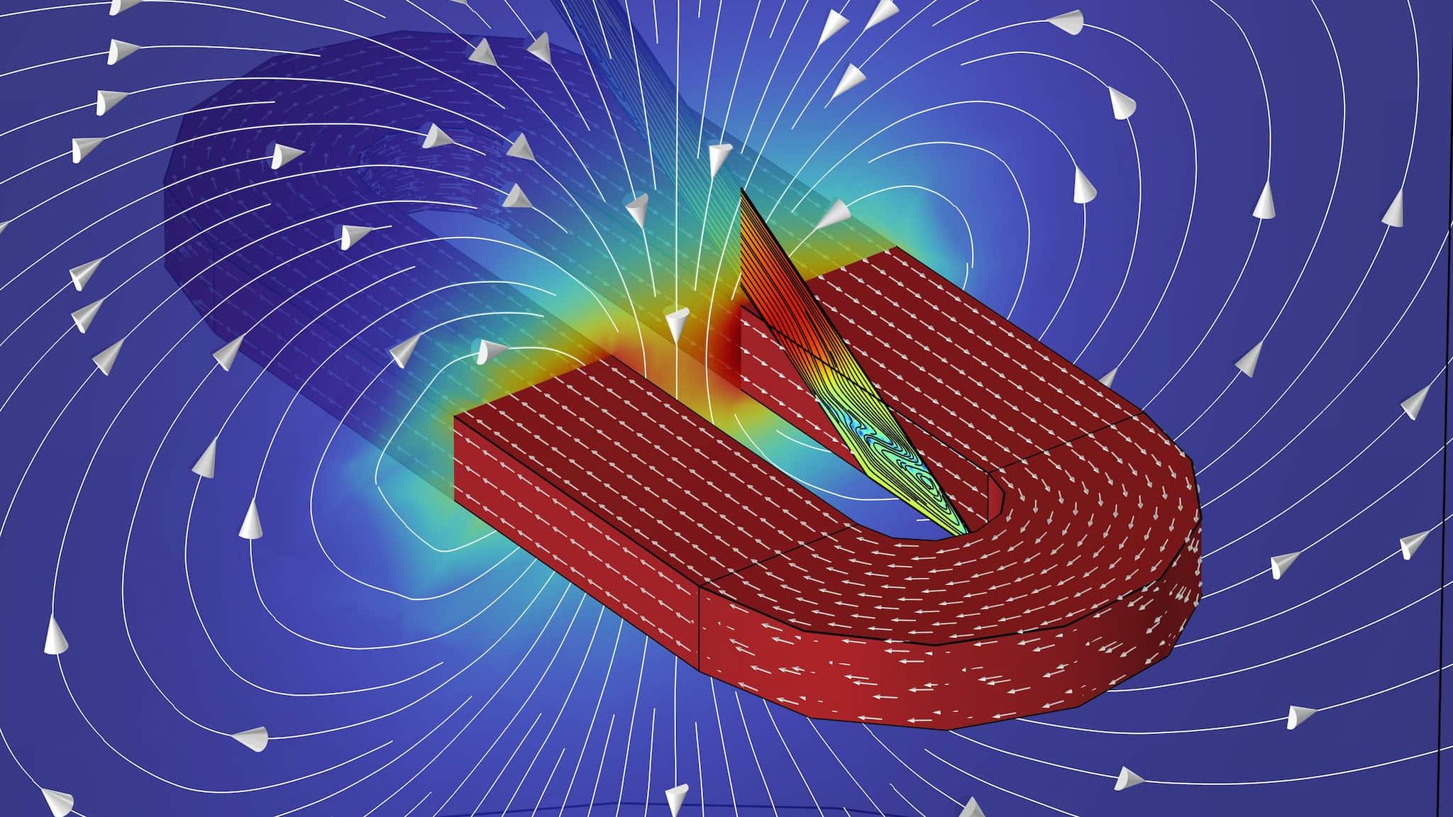
Superconducting coils are used to generate high magnetic fields in various applications such as nuclear fusion reactors, particle accelerators, actuators and MRI scanners. In all of these cases, the current density that is required for the necessary field strength exceeds the practical limits of regular coils. At the same time, the physics of the superconductor itself is strongly influenced by the external magnetic field that is generated by the coil. Modelling superconductors using FEM can be utilized to predict e.g. the current distribution, the critical current, the magnetic field and AC losses. Here, we studied the case of a single superconducting coil and the influence of its magnetic field on the current distribution and critical current in the superconducting tape that is feeding it (the lead). Our novel approach allows the simultaneous computation of magnetic field, current and voltage inside the superconductor.
Different angles between the lead and the coil
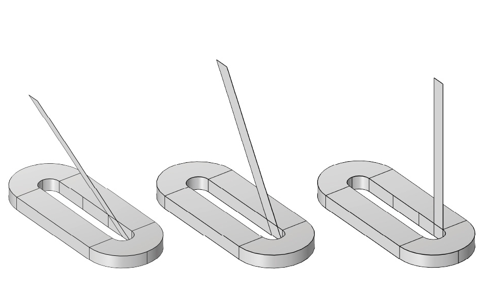
To determine the critical current in the superconducting lead cable, the current inside of the coil is not relevant. We only need to know the effect of the magnetic field generated by the coil on the superconducting wire. The geometry is sketched in the figure below. We show three different geometries, each with a different angle of the incoming lead (30°, 60° and 90°). This angle is important, because of the functional relationship that exists between the critical current in the superconductor (which is the current at which the superconductor starts to show a significant voltage drop) and the external magnetic field. One may conceptualize the critical current suppression in the superconductor as the result of a Lorentz force of the charged superconducting particles (Cooper pairs) on the flux vortices, so that when the current and the magnetic field are perpendicular, the resulting suppression of the critical current is maximal. This point is reached close to the top of the coil. We were interested in how the supercurrent is distributed throughout the superconducting lead cable and how the suppression in the critical current in the lead close to the coil are affected by the angle of incidence.
modelling superconductors
a modified AV-formulation.
Electrodynamic modelling of superconductors is challenging because of the significant nonlinearity in the electric field – current (E(J)) relation. In contrast to regular conductors, where the electric field and current are linearly dependent variables (i.e. Ohm’s law), the superconductor E(J) curve is E(J) = EC (J/JC)n with n ≈ 20. As a result, the usual modelling strategies for solving Maxwell’s equations must be modified, in order to converge the simulation at all. These strategies are named after the dependent variables in Maxwell’s equations that is being solved for. For instance, conventional electromagnetic simulations solve for the scalar electrical potential V and the magnetic vector potential A, earning the name AV-formulation. It is possible to model superconductors using AV as well, but undesirable modifications to the E(J)-relation must be made. The conventional method for modelling superconductors thus involves other formulations, where the correct E(J) curve can be used. The most prominent and simple is the H-formulation, where the magnetic H-field is the dependent variable and the current is given by its curl, as follows from Ampère’s law. The downside of the conventional superconductor modelling formulations is that the voltage is usually not readily available in the simulations and if it is, it is only in lumped form. We have modified the AV-formulation to get the best of both worlds: spatially resolved voltages as well as the correct E(J) curve.
the effective critical current of the lead.
The AV-formulation allows us direct access to the voltage drop over the superconducting lead. The current inside the coil is modelled as the number of turns times the current that is flowing through the lead. The coil thus acts as an external current density that generates a magnetic field; its superconducting properties are not relevant and not directly modelled. The lead and coil are connected by a soldered interface which is taken into account in the simulation. This is necessarily a metallic (non-superconducting) interface, which introduces an Ohmic term into the voltage drop over the entire lead. As there is access to the spatially resolved voltage (thanks to the modified AV-formalism), it is possible to obtain the voltage drop over the superconducting tape only. The end result is that we have unambiguous, reliable numerical results for the voltage drop over the superconducting lead as a function of the applied current. This directly allows us to find the effective critical current (defined to be the current value at which the critical E-field at 1·10-4 V/m is reached) of the entire lead.
Results
current distribution and critical current in the lead.
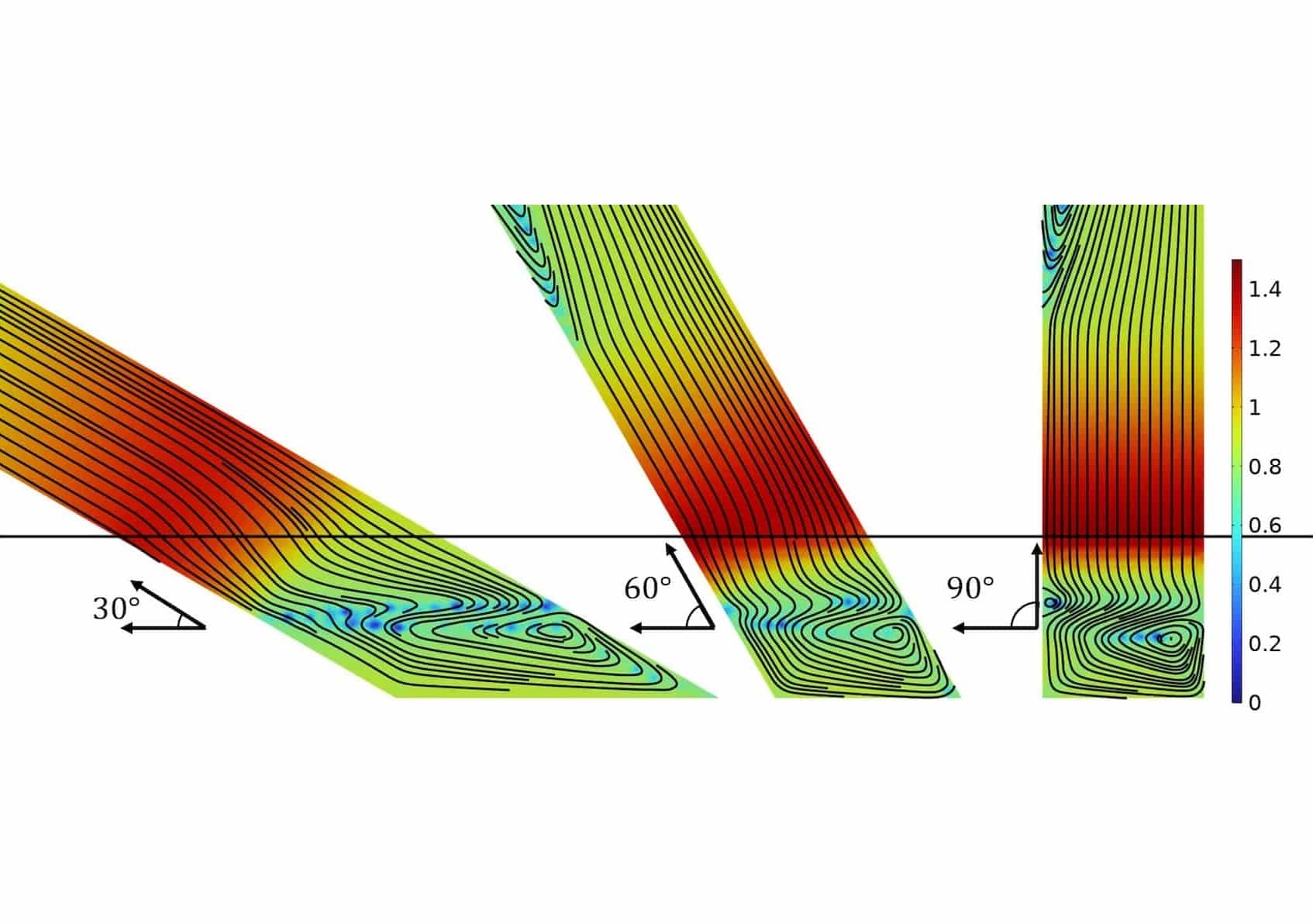
The figure above shows the supercurrent distribution inside the lead close to the coil, in dimensionless units of Js/Jc. The horizontal black line indicates the top of the coil. The black streamline pattern showing the direction of the current is similar for the three different angles of incidence, but stretched out over a surface with different aspect ratio. Additionally, the supercurrent can be seen to cross the line where the tape meets the coil as perpendicularly as possible, deviating from the straight line it was following before that point. It is along this black line that the critical current is at its lowest value, as also seen the figure on the left. Another interesting feature of the critical current as shown on the left is the maximum that is attained precisely halfway through the coil. At this point, the symmetry of the coil mandates that the magnetic field lines are perfectly parallel to the lead, resulting in a strong local variation in Jc.
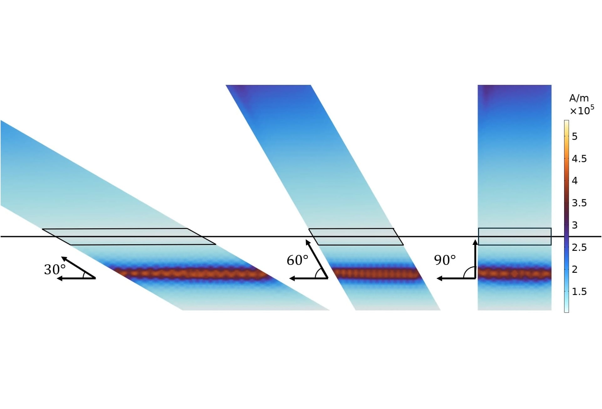
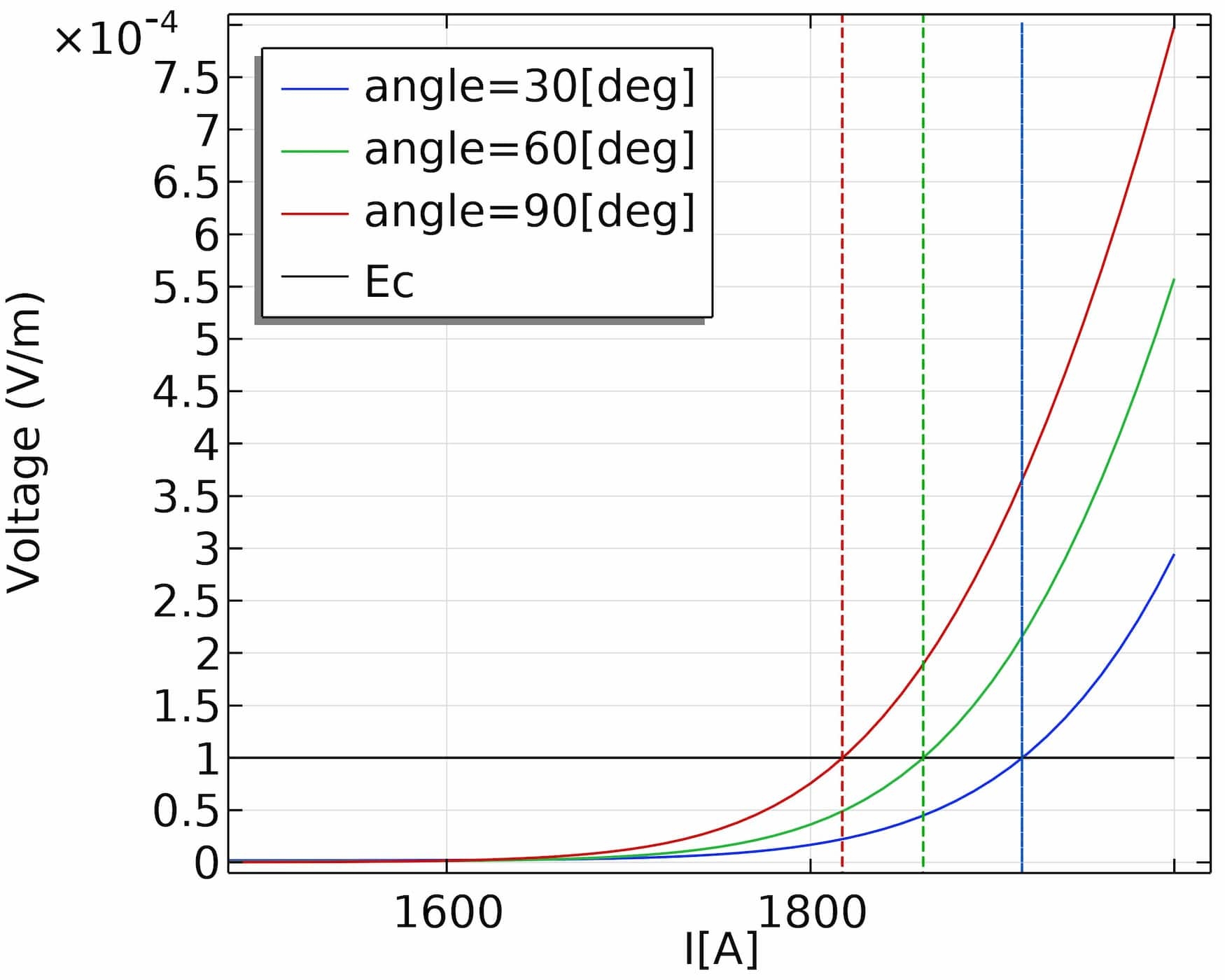
The modified AV-formulation allows the usage of current terminals, so that we directly have access to the voltage drop over the superconducting lead. The plot below shows the electric field – current relation of the superconducting lead for the three different angles of incidence. Notably, the effective critical current of the lead changes with the angle of incidence, showing that not only does the current distribution change, the voltage drop (or electric field) does as well. The highest effective critical current is obtained when the angle between the lead and the coil is 30°, which out of the three cases shown here maximizes the area at which the critical current is at its minimum (see parallellograms in Figure 3).
conclusion.
We have successfully modelled a superconducting lead connected to a coil, showing the effect of changing the angle of incidence of the lead on the current distribution inside the lead, the critical current inside the lead and the effective critical current of the total lead. The latter could be done very easily because of our modified AV-formulation, which allows direct access to the voltage, while keeping the correct E(J)-relation so that the physics is unaffected.
In conclusion, we showed an example of modelling superconductors, including current sharing and voltages, directly predicting properties of superconducting device designs. The modelling is of direct use in engineering, since knowledge about the critical current of a superconducting device is vital to the design. Moving the discovery of such knowledge from experiment to simulation greatly reduces costs and increases the fundamental insights tremendously.
"building, developing and improving technology is what makes us engineers"
Computational superconductivity presents a very satisfying combination of exotic physics, high-tech application and technically challenging computations. Improving the simulation methodology to allow for a more accurate description of the physics is especially rewarding. The ultimate goal of our work is to build, develop and improve technology – this is what makes us engineers!